Distinguishing pure diffusions from jump-diffusions
One important question when we have some time series – possibly from real-world data – is to be able to discern if this timeseries is a pure diffusion process (a continuous stochastic process) or a jump-diffusion process (a discontinuous stochastic process).
For this, jumpdiff has an easy to use function, called q_ratio.
The idea behind distinguishing continuous and discontinuous processes is simple:
diffusion processes diffuse over time, thus they take time to occupy space; jump-diffusion processes can jump, and thus statistically, they occupy all space very fast.
To analyse this let us design a simple example – with some numerically generated data – that shows the use of q_ratio and how to read it.
Let us generate two trajectories, using jd_process, denoted d_timeseries and j_timeseries, for diffusion timeseries and jumpy timeseries.
Naturally the first must not include a jump term.
To keep it simple, we will use the same parameters for both, expect for the jumps:
1 2 3 4 5 6 7 8 9 10 11 12 13 14 15 16 17 | import jumpdiff as jd # integration time and time sampling t_final = 10000 delta_t = 0.01 # Drift function def a(x): return -0.5*x # Diffusion function def b(x): return 0.75 # generate 2 trajectories d_timeseries = jd.jd_process(t_final, delta_t, a=a, b=b, xi=0, lamb=0) j_timeseries = jd.jd_process(t_final, delta_t, a=a, b=b, xi=2.5, lamb=1.75) |
Note how xi and lamb are different for each process
To now examine the rate of diffusion of the processes, we need to generate a time arrow, which we denote lag.
This needs to be a integer list >0.
18 19 | import numpy as np lag = np.logspace(0, 3, 25, dtype=int) |
Lastly we just need to can the q_ratio for our two timeseries
20 21 | d_lag, d_Q = jd.q_ratio(lag, d_timeseries) j_lag, j_Q = jd.q_ratio(lag, j_timeseries) |
And with the help of matplotlib’s plotly, we can visualise the results in a double logarithmic scale
22 23 24 25 | import matplotlib.plotly as plt plt.loglog(d_lag, d_Q, '-', label='diffusion') plt.loglog(j_lag, j_Q, 'o-', label='jump-diffusion') |
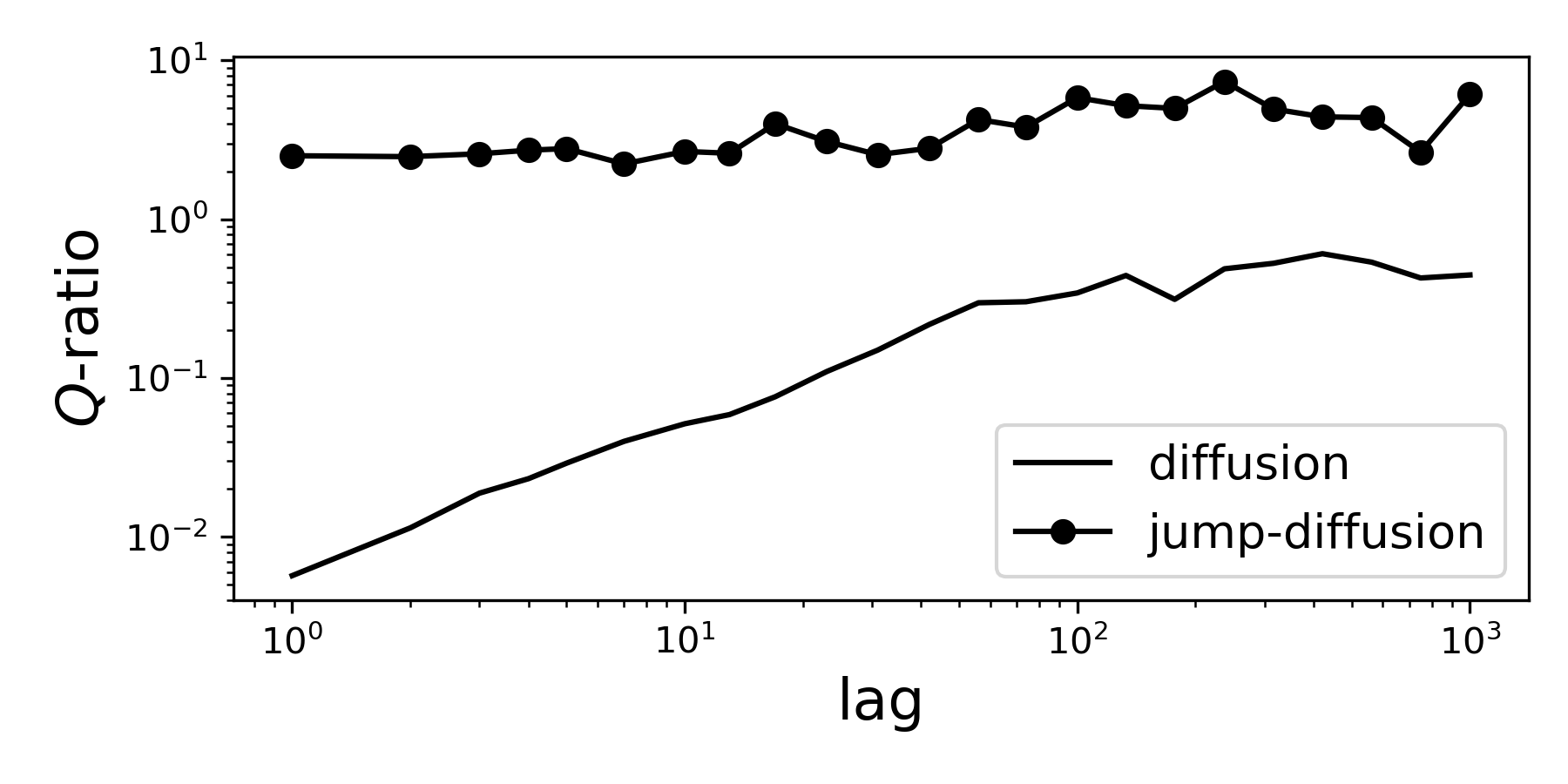
As we can see, the diffusion process grows with our time arrow lag, where the jump-diffusion is constant (does not depend on lag).
Jump processes will show a constant relation with code:lag, where diffusion processes a linear relation.