Jump-diffusion processes

The theory

Jump-diffusion processes¹, as the name suggest, are a mixed type of stochastic processes with a diffusive and a jump term. One form of these processes which is mathematically traceable is given by the Stochastic Differential Equation

\[\mathrm{d} X(t) = a(x,t)\;\mathrm{d} t + b(x,t)\;\mathrm{d} W(t) + \xi\;\mathrm{d} J(t),\]

which has four main elements: a drift term \(a(x,t)\), a diffusion term \(b(x,t)\), linked with a Wiener process \(W(t)\), a jump amplitude term \(\xi(x,t)\), which is given by a Gaussian distribution \(\mathcal{N}(0,\sigma_\xi^2)\) coupled with a jump rate \(\lambda\), which is the rate of the Poissonian jumps \(J(t)\). You can find a good review on this topic in Ref. 2.

Integrating a jump-diffusion process

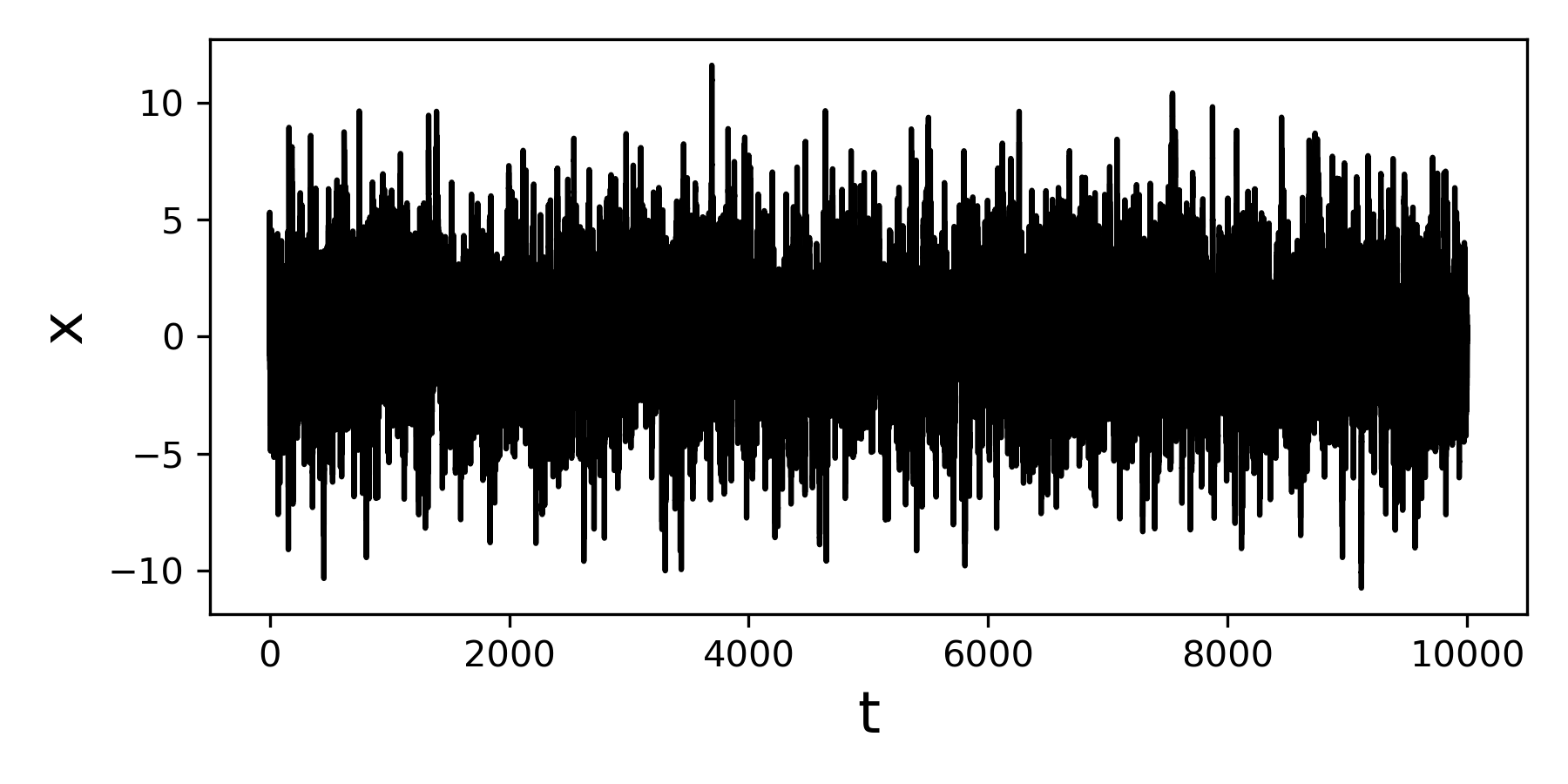
Let us use the functions in JumpDiff to generate a jump-difussion process, and subsequently retrieve the parameters. This is a good way to understand the usage of the integrator and the non-parametric retrieval of the parameters.

First we need to load our library. We will call it jd

import JumpDiff as jd

Let us thus define a jump-diffusion process and use jdprocess to integrate it. Do notice here that we need the drift \(a(x,t)\) and diffusion \(b(x,t)\) as functions.

# integration time and time sampling
t_final = 10000
delta_t = 0.001

# A drift function
def a(x):
    return -0.5*x

# and a (constant) diffusion term
def b(x):
    return 0.75

# Now define a jump amplitude and rate
xi = 2.5
lamb = 1.75

# and simply call the integration function
X = jd.jdprocess(t_final, delta_t, a=a, b=b, xi=xi, lamb=lamb)

This will generate a jump diffusion process X of length int(10000/0.001) with the given parameters.

Using JumpDiff to retrieve the parameters

Moments and Kramers─Moyal coefficients

Take the timeseries X and use the function moments to retrieve the conditional moments of the process. For now let us focus on the shortest time lag, so we can best approximate the Kramers—Moyal coefficients. For this case we can simply employ

edges, moments = jd.moments(timeseries = X)

In the array edges are the limits of our space, and in our array moments are recorded all 6 powers/order of our conditional moments. Let us take a look at these before we proceed, to get acquainted with them.

We can plot the first moment with any conventional plotter, so lets use here plotly from matplotlib

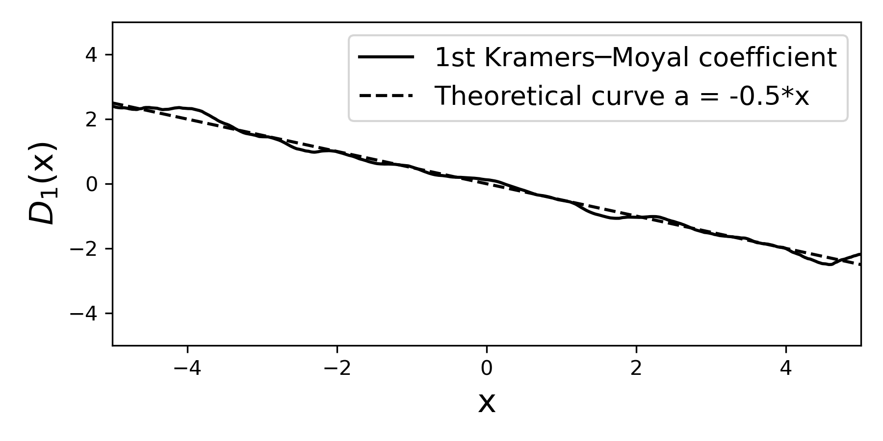
The first moment here (i.e., the first Kramers—Moyal coefficient) is given solely by the drift term that we have selected -0.5*x

And the second moment (i.e., the second Kramers—Moyal coefficient) is a mixture of both the contributions of the diffusive term \(b(x)\) and the jump terms \(\xi\) and \(\lambda\).

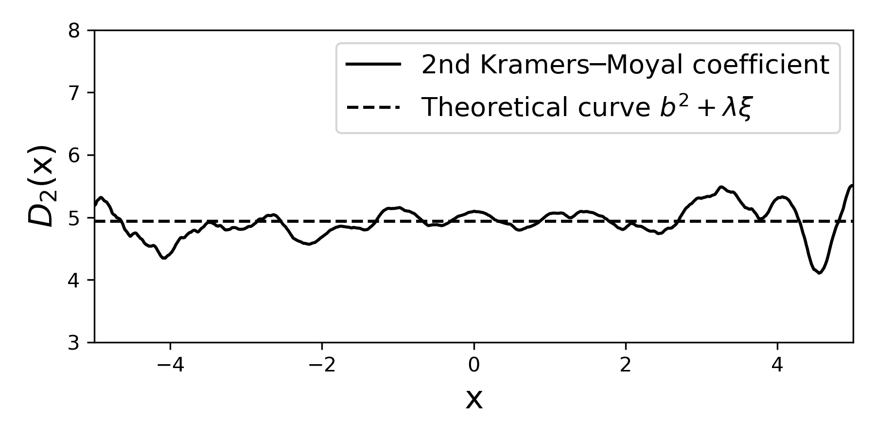
You have this stored in moments[2,...].

Retrieving the jump-related terms

Naturally one of the most pertinent questions when addressing jump-diffusion processes is the possibility of recovering these same parameters from data. For the given jump-diffusion process we can use the jump_amplitude and jump_rate functions to non-parametrically estimate the jump amplitude \(\xi\) and \(\lambda\) terms.

After having the moments in hand, all we need is

# first estimate the jump amplitude
xi_est = jd.jump_amplitude(moments = moments)

# and now estimated the jump rate
lamb_est = jd.jump_rate(moments = moments)

which resulted in our case in (xi_est) ξ = 2.43 ± 0.17 and (lamb_est) λ = 1.744 * delta_t (don’t forget to divide lamb_est by delta_t)!

Other functions and options

Include in this package is also the Milstein scheme of integration, particularly important when the diffusion term has some spacial x dependence. moments can actually calculate the conditional moments for different lags, using the parameter lag.

In formulae the set of formulas needed to calculate the second order corrections are given (in sympy).