jumpdiff

jumpdiff is a python library with non-parametric Nadaraya—Watson estimators to extract the parameters of jump-diffusion processes. With jumpdiff one can extract the parameters of a jump-diffusion process from one-dimensional timeseries, employing both a kernel-density estimation method combined with a set on second-order corrections for a precise retrieval of the parameters for short timeseries.

Installation

To install jumpdiff simply use

pip install jumpdiff

Then on your favourite editor just use

import jumpdiff as jd

The library depends on numpy, scipy, and sympy.

Jump-diffusion processes

We will show here how to: (1) generate trajectories of jump-diffusion processes; (2) retrieve the parameters from a single trajectory of a jump-diffusion process. Naturally, if we already had some data – maybe from a real-world recording of a stochastic process – we would simply look at estimating the parameters for this process.

The theory

Jump-diffusion processes¹, as the name suggest, are a mixed type of stochastic processes with a diffusive and a jump term. One form of these processes which is mathematically traceable is given by the Stochastic Differential Equation

\[\mathrm{d} X(t) = a(x,t)\;\mathrm{d} t + b(x,t)\;\mathrm{d} W(t) + \xi\;\mathrm{d} J(t),\]

which has four main elements: a drift term \(a(x,t)\), a diffusion term \(b(x,t)\), linked with a Wiener process \(W(t)\), a jump amplitude term \(\xi(x,t)\), which is given by a Gaussian distribution \(\mathcal{N}(0,\sigma_\xi^2)\) coupled with a jump rate \(\lambda\), which is the rate of the Poissonian jumps \(J(t)\). You can find a good review on this topic in Ref. 2.

Integrating a jump-diffusion process

Let us use the functions in jumpdiff to generate a jump-difussion process, and subsequently retrieve the parameters. This is a good way to understand the usage of the integrator and the non-parametric retrieval of the parameters.

First we need to load our library. We will call it jd

import jumpdiff as jd

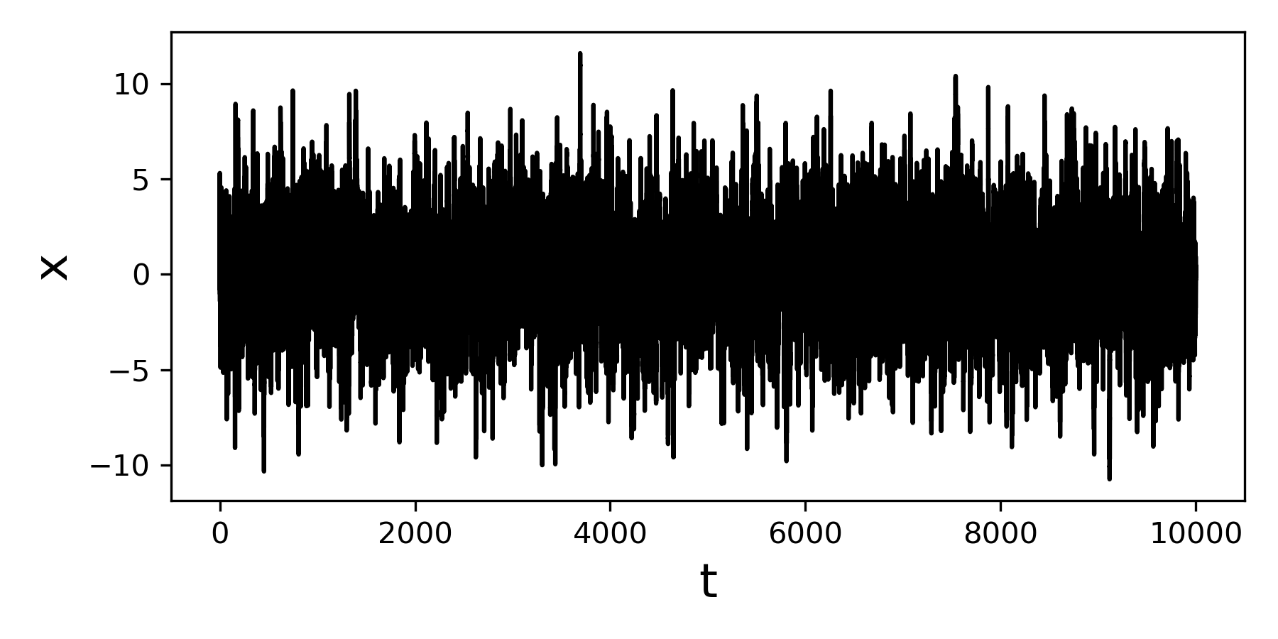
Let us thus define a jump-diffusion process and use jd_process to integrate it. Do notice here that we need the drift \(a(x,t)\) and diffusion \(b(x,t)\) as functions.

# integration time and time sampling
t_final = 10000
delta_t = 0.001

# A drift function
def a(x):
    return -0.5*x

# and a (constant) diffusion term
def b(x):
    return 0.75

# Now define a jump amplitude and rate
xi = 2.5
lamb = 1.75

# and simply call the integration function
X = jd.jd_process(t_final, delta_t, a=a, b=b, xi=xi, lamb=lamb)

This will generate a jump diffusion process X of length int(10000/0.001) with the given parameters.

Using jumpdiff to retrieve the parameters

Moments and Kramers─Moyal coefficients

Take the timeseries X and use the function moments to retrieve the conditional moments of the process. For now let us focus on the shortest time lag, so we can best approximate the Kramers—Moyal coefficients. For this case we can simply employ

edges, moments = jd.moments(timeseries = X)

In the array edges are the limits of our space, and in our array moments are recorded all 6 powers/order of our conditional moments. Let us take a look at these before we proceed, to get acquainted with them.

We can plot the first moment with any conventional plotter, so lets use here plotly from matplotlib. To visualise the first moment, simply use

import matplotlib.pyplot as plt
plt.plot(edges, moments[1]/delta_t)

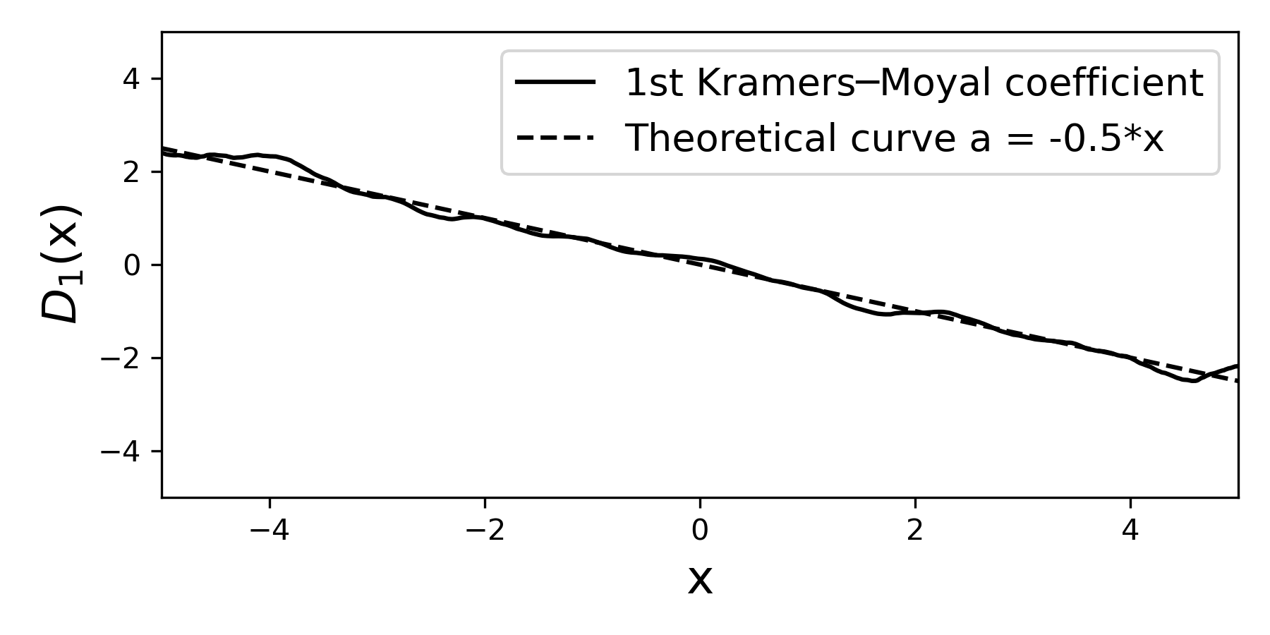
The first moment here (i.e., the first Kramers—Moyal coefficient) is given solely by the drift term that we have selected -0.5*x. In the plot we have also included the theoretical curve, which we know from having selected the value of a(x) in line 8.

Similarly, we can extract the second moment (i.e., the second Kramers—Moyal coefficient) is a mixture of both the contributions of the diffusive term \(b(x)\) and the jump terms \(\xi\) and \(\lambda\).

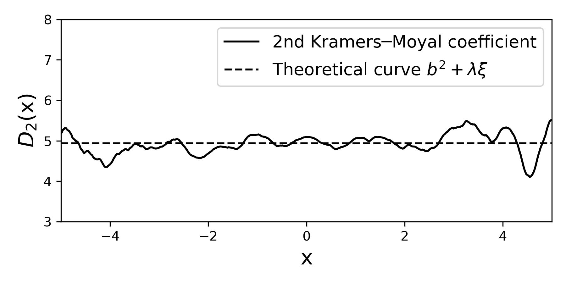
You have this stored in moments[2].

Retrieving the jump-related terms

Naturally one of the most pertinent questions when addressing jump-diffusion processes is the possibility of recovering these same parameters from data. For the given jump-diffusion process we can use the jump_amplitude and jump_rate functions to non-parametrically estimate the jump amplitude \(\xi\) and \(\lambda\) terms.

After having the moments in hand, all we need is

# first estimate the jump amplitude
xi_est = jd.jump_amplitude(moments = moments)

# and now estimated the jump rate
lamb_est = jd.jump_rate(moments = moments)

which resulted in our case in (xi_est) ξ = 2.43 ± 0.17 and (lamb_est) λ = 1.744 * delta_t (don’t forget to divide lamb_est by delta_t)! We can compare these with our chose values in lines 15-16.

Distinguishing pure diffusions from jump-diffusions

One important question when we have some time series – possibly from real-world data – is to be able to discern if this timeseries is a pure diffusion process (a continuous stochastic process) or a jump-diffusion process (a discontinuous stochastic process). For this, jumpdiff has an easy to use function, called q_ratio. The idea behind distinguishing continuous and discontinuous processes is simple: diffusion processes diffuse over time, thus they take time to occupy space; jump-diffusion processes can jump, and thus statistically, they occupy all space very fast.

To analyse this let us design a simple example – with some numerically generated data – that shows the use of q_ratio and how to read it.

Let us generate two trajectories, using jd_process, denoted d_timeseries and j_timeseries, for diffusion timeseries and jumpy timeseries. Naturally the first must not include a jump term. To keep it simple, we will use the same parameters for both, expect for the jumps:

import jumpdiff as jd

# integration time and time sampling
t_final = 10000
delta_t = 0.01

# Drift function
def a(x):
    return -0.5*x

# Diffusion function
def b(x):
    return 0.75

# generate 2 trajectories
d_timeseries = jd.jd_process(t_final, delta_t, a=a, b=b, xi=0, lamb=0)
j_timeseries = jd.jd_process(t_final, delta_t, a=a, b=b, xi=2.5, lamb=1.75)

Note how xi and lamb are different for each process To now examine the rate of diffusion of the processes, we need to generate a time arrow, which we denote lag. This needs to be a integer list >0.

import numpy as np
lag = np.logspace(0, 3, 25, dtype=int)

Lastly we just need to can the q_ratio for our two timeseries

d_lag, d_Q = jd.q_ratio(lag, d_timeseries)
j_lag, j_Q = jd.q_ratio(lag, j_timeseries)

And with the help of matplotlib’s plotly, we can visualise the results in a double logarithmic scale

import matplotlib.plotly as plt

plt.loglog(d_lag, d_Q, '-', label='diffusion')
plt.loglog(j_lag, j_Q, 'o-', label='jump-diffusion')

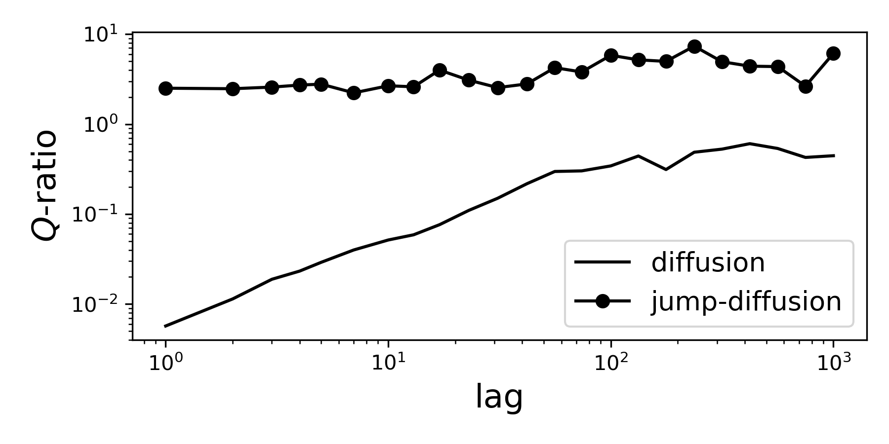
As we can see, the diffusion process grows with our time arrow lag, where the jump-diffusion is constant (does not depend on lag). Jump processes will show a constant relation with code:lag, where diffusion processes a linear relation.

Table of Content

• Installation
• Jump-diffusion processes
  • The theory
  • Integrating a jump-diffusion process
  • Using jumpdiff to retrieve the parameters
    • Moments and Kramers─Moyal coefficients
    • Retrieving the jump-related terms
• Distinguishing pure diffusions from jump-diffusions
• Functions
  • Jump-diffusion timeseries generator
  • Moments
  • Parameters
  • Q-ratio
  • Formulae
  • Helping functions
    • Kernels function
• License
• Contact

Literature

¹ Tabar, M. R. R. Analysis and Data-Based Reconstruction of Complex Nonlinear Dynamical Systems. Springer, International Publishing (2019), Chapter Stochastic Processes with Jumps and Non-vanishing Higher-Order Kramers—Moyal Coefficients*.

² Friedrich, R., Peinke, J., Sahimi, M., Tabar, M. R. R. Approaching complexity by stochastic methods: From biological systems to turbulence, Physics Reports 506, 87–162 (2011).

³ Rydin Gorjão, L., Meirinhos, F. kramersmoyal: Kramers–Moyal coefficients for stochastic processes. Journal of Open Source Software, 4(44) (2019).

An extensive review on the subject can be found here.

Funding

Helmholtz Association Initiative Energy System 2050 - A Contribution of the Research Field Energy and the grant No. VH-NG-1025 and STORM - Stochastics for Time-Space Risk Models project of the Research Council of Norway (RCN) No. 274410.